 加载中…
加载中…FRM(17)BSM model
标签:
杂谈 |
分类: CrewsHE |
Black–Scholes model
The Black–Scholes model of the market for a particular equity
makes the following explicit assumptions:
- It is possible to borrow and lend cash at a known constant risk-free interest rate.
- The price follows a geometric Brownian motion with constant drift and volatility.
- There are no transaction costs.
- The stock does not pay a dividend (see below for extensions to handle dividend payments).
- All securities are perfectly divisible (i.e. it is possible to buy any fraction of a share).
- There are no restrictions on short selling.
- There is no arbitrage opportunity
From these ideal conditions in the market for an equity (and
for an option on the equity), the authors show that "it is possible
to create a hedged
position, consisting of a long position in the stock and a
short position in [calls on the same stock], whose value will not
depend on the price of the stock."[2]"
Notation
Define
- S, the price of the stock (please note as below).
- V(S,t), the price of a derivative as a function of time and stock price.
- C(S,t) the price of a European call and P(S,t) the price of a European put option.
- K, the strike of the option.
- r, the annualized risk-free interest rate, continuously compounded.
- μ, the drift rate of S, annualized.
- σ, the volatility of the stock; this is the square root of the quadratic variation of the stock’s log price process.
- t a time in years; we generally use now = 0, expiry = T.
- Π, the value of a portfolio.
- R, the accumulated profit or loss following a delta-hedging trading strategy.
N(x) denotes the standard
normalcumulative
distribution function, http://upload.wikimedia.org/math/6/3/d/63dde1ffc859af893749b19f47b53b28.pngmodel" />.
N‘(x) denotes the standard normal
probability density function,http://upload.wikimedia.org/math/9/0/a/90af1f9a083bc2ac16d223def39ed1d5.pngmodel" />.
Black–Scholes PDE
http://upload.wikimedia.org/wikipedia/commons/thumb/f/f2/Stockpricesimulation.jpg/180px-Stockpricesimulation.jpgmodel" />
Simulated Geometric Brownian Motions with Parameters from
Market Data
As per the model assumptions above, we assume that the
underlying
asset (typically the stock) follows a
geometric Brownian motion. That is,
where Wt is Brownian—the dW
term here stands in for any and all sources of uncertainty in the
price history of a stock.
The payoff of an option
V(S,T) at maturity is known. To
find its value at an earlier time we need to know how V
evolves as a function of S and T. By Itō’s
lemma for two variables we have
Now consider a trading strategy under which one holds a single
option and continuously trades in the stock in order to hold
http://upload.wikimedia.org/math/a/9/1/a9140b87bacbd1cc819b3f3d64bf68ba.pngmodel" /> shares. At time t, the value of these holdings
will be
The composition of this portfolio, called the delta-hedge
portfolio, will vary from time-step to time-step. Let R
denote the accumulated profit or loss from following this strategy.
Then over the time period [t, t + dt], the
instantaneous profit or loss is
By substituting in the equations above we get
This equation contains no dW term. That is, it is
entirely riskless (delta
neutral). Black and Scholes reason that under their ideal
conditions, the rate of return on this portfolio must be equal at
all times to the rate of return on any other riskless instrument;
otherwise, there would be opportunities for arbitrage.
Now assuming the risk-free rate of return is r we must have
over the time period [t, t + dt]
If we now substitute in for Π and divide through
by dt we obtain the Black–Scholes
PDE:
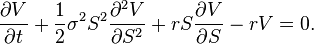
With the assumptions of the Black–Scholes model, this partial
differential equation holds whenever V is twice
differentiable with respect to S and once with respect to
t.
Above we used the method of arbitrage-free
pricing ("delta-hedging")
to derive some PDE governing option prices given the Black–Scholes
model. It is also possible to use a
risk-neutrality argument. This latter method gives the price as
the expectation
of the option payoff under a particular probability
measure, called the
risk-neutral measure, which differs from the real world
measure.
Black–Scholes formula
http://upload.wikimedia.org/wikipedia/commons/thumb/1/12/Optionpricesurface.jpg/180px-Optionpricesurface.jpgmodel" />
Black-Scholes European Call Option Pricing Surface
The Black Scholes formula is used for obtaining the price of
Europeanput
and call
options. It is obtained by solving the Black–Scholes PDE as
discussed – see derivation below.
The value of a call option in terms of the Black–Scholes
parameters:
The price of a put
option is:
For both, as
above:
- N(•) is the standard normal or cumulative distribution function
- T – t is the time to maturity
- S is the spot price of the underlying asset
- K is the strike price
- r is the risk free rate (annual rate, expressed in terms of continuous compounding)
- σ is the volatility in the log-returns of the underlying
Interpretation
N(d1) and
N(d2) are the probabilities
of the option expiring in-the-money under the equivalent
exponential
martingale probability measure (numéraire
= stock) and the equivalent martingale probability measure
(numéraire = risk free asset), respectively. The equivalent
martingale probability measure is also called the risk-neutral
probability measure. Note that both of these are
probabilities in a
measure theoretic sense, and neither of these is the true
probability of expiring in-the-money under the real probability
measure.
Derivation
We now show how to get from the general Black–Scholes PDE to a
specific valuation for an option. Consider as an example the
Black–Scholes price of a call
option, for which the PDE above has boundary
conditions
The last condition gives the value of the option at the time
that the option matures. The solution of the PDE gives the value of
the option at any earlier time, http://upload.wikimedia.org/math/3/2/7/327c39b2c927a4afc20a742898d4932b.pngmodel" />. In order to solve the PDE we transform the equation
into a diffusion
equation which may be solved using standard methods. To this
end we introduce the change-of-variable transformation
Then the Black–Scholes PDE becomes a diffusion equation
The terminal condition C(S,T) =
max(S− K,0) now becomes an initial
condition
Using the standard method for solving a diffusion equation we
have
After some algebra we obtain
where
and
Substituting for u, x, and τ, we
obtain the value of a call option in terms of the Black–Scholes
parameters:
where
The price of a put
option may be computed from this by put-call
parity and simplifies to
- http://upload.wikimedia.org/math/1/d/b/1dbe1d65b864ee9a63ef9ded7df9f044.pngmodel" />
- BS模型的理解:
- bs模型,一个让人又爱又恨的model,开始入门的时候,觉得这个模型简直就是天才的杰作,虽然说看着公式复杂,其实计算还是很简单的,那么一折腾就能得到想要的结果,最重要的是这个结果还不算太坏。于是很是兴奋的拿着公式满世界挥舞,却发现这也不行,那也不行,一时间完全失去了对这些个模型的信心。
- 后来慢慢看见的模型多了,开始慢慢理解bs了。 我曾经和bobo说过,虽然我们用着bs,其实bs的含义是很简单的,就是一个有价值的部分的实现加权加上一个没有价值部分的不实现加权。这样理解的话,那些歌N(D1)和N(d2)就变成了纯粹的概率问题,我们在用正态的时候这个值可能容易算出来,可是要是把这个过程看成其他的分布就难了。假设这个过程是一个power-law的过程,假设这个power-law的a和效用函数是有关系的,这个a和市场也是有关系的,怎么样得到一个简单的表达和一个完整的推导?假设这个过程是一个levy process,比如说是VG,是CGMY,怎么样求那个default的概率,这又是一大堆问题了,有空我真想把power-law的那个想法做一下,不过现在看起来要等这个考试结束了。
- anyway,看习题,写习题,这一章没有难点,难点我也基本搞定了。过。
![]() 喜欢
喜欢
0
![]() 赠金笔
赠金笔