加好友 发纸条
写留言 加关注
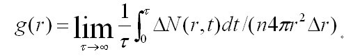
径向分布函数g(r)代表了球壳内的平均数密度 http://pic.muchong.com/201009/13/664177_194049.jpg 为离中心分子距离为r,体积为 的球壳内的瞬时分子数。 具体参见李如生,《平衡和非平衡统计力学》科学出版社:1995
Here are the computer codes for this article:
md_rdf.cpp
find_rdf.m
test_rdf.m
Calculating radial distribution function in molecular dynamics
http://image.sciencenet.cn/home/201711/08/071400tvog6so2lfp666hb.jpg
First I recommend a very good book on molecular dynamics (MD) simulation: the book entitled "Molecular dynamics simulation: Elementary methods" by J. M. Haile. I read this book 7 years ago when I started to learn MD simulation, and recently I enjoyed a second reading of this fantastic book. If a beginner askes me which book he/she should read about MD, I will only recommend this. This is THE BEST introductory book on MD. It tells you what is model, what is simulation, what is MD simulation, and what is the correct attitude for doing MD simulations.
In my last blog article, I have presented a Matlab code for calculating velocity autocorrelation function (VACF) and phonon density of states (PDOS) from saved velocity data. In this article, I will present a Matlab code for calculating the radial distribution function (RDF) from saved position data. The relevant definition and algorithm are nicely presented in Section 6.4 and Appendix A of Haile's book. Here I only present a C code for doing MD simulation and a Matlab code for calculating and plotting the RDF. We aim to reproduce Fig. 6.22 in Haile's book!
Step 1.
Use the C code provided above to do an MD simulation. Note that I have used a different unit systems than that used in Haile's book (he used the LJ unit system). This code only takes 14 seconds to run in my desktop. Here are my position data (there are 100 frames and each frame has 256 atoms):
r.txt
Step 2.
Write a Matlab function which can calculate the RDF for one frame of positions:
function [g] = find_rdf(r, L, pbc, Ng, rc)
% determine some parameters
N = size(r, 1); % number of particles
L_times_pbc = L .* pbc; % deal with boundary conditions
rho = N / prod(L); % global particle density
dr = rc / Ng; % bin size
% accumulate
g = zeros(Ng, 1);
for n1 = 1 : (N - 1) % sum over the atoms
for n2 = (n1 + 1) : N % skipping half of the pairs
r12 = r(n2, :) - r(n1, :); % position difference vector
r12 = r12 - round(r12 ./L ) .* L_times_pbc; % minimum image convention
d12 = sqrt(sum(r12 .* r12)); % distance
if d12 < rc % there is a cutoff
index = ceil(d12 / dr); % bin index
g(index) = g(index) + 1; % accumulate
end
% normalize
for n = 1 : Ng
g(n) = g(n) / N * 2; % 2 because half of the pairs have been skipped
dV = 4 * pi * (dr * n)^2 * dr; % volume of a spherical shell
g(n) = g(n) / dV; % now g is the local density
g(n) = g(n) / rho; % now g is the RDF
Step 3.
Write a Matlab script to load the position data, call the function above, and plot the results:
clear; close all;
load r.txt; % length in units of Angstrom
% parameters from MD simulation
N = 256; % number of particles
L = 5.60 * [4, 4, 4]; % box size
pbc = [1, 1, 1]; % boundary conditions
% number of bins (number of data points in the figure below)
Ng = 100;
% parameters determined automatically
rc = min(L) / 2; % the maximum radius
Ns = size(r, 1) / N; % number of frames
% do the calculations
g = zeros(Ng, 1); % The RDF to be calculated
for n = 1 : Ns
r1 = r(((n - 1) * N + 1) : (n * N), :); % positions in one frame
g = g + find_rdf(r1, L, pbc, Ng, rc); % sum over frames
g = g / Ns; % time average in MD
% plot the data
r = (1 : Ng) * dr / 3.405;
figure;
plot(r, g, 'o-');
xlim([0, 3.5]);
ylim([0, 3.5]);
xlabel('r^{\ast}', 'fontsize', 15)
ylabel('g(r)', 'fontsize', 15)
set(gca, 'fontsize', 15);
Here is the figure I obtained:
http://image.sciencenet.cn/home/201711/08/070243krljlglcu2fhaak0.png
Does it resemble Fig. 6. 22 in Haile's book?
https://www.cnblogs.com/Simulation-Campus/p/8994935.html
喜欢
0
赠金笔
 加载中…
加载中…