 加载中…
加载中…Overhauser (Catmull-Rom) Splines for Camera Animation
标签:
样条曲线cit |
分类: 学习笔记 |
此文转自如下网址:
http://www.codeproject.com/Articles/30838/Overhauser-Catmull-Rom-Splines-for-Camera-Animatio
Introduction
Many people are impressed by realistic camera animations in games or multimedia demos. The math behind what is commonly called camera interpolation is actually pretty simple. In this article, I will focus on a simple algorithm that uses a particular class of spline curves called Overhauser or Catmull-Rom splines, and I will show how and why they are superior to other existing more or less similar approaches.
Math is Your Friend
You may hate me for this, but math can be really nice. We will brush up our knowledge of vector calculus in this section, which will allow us to understand the sample code better.
Let's start with the basics: A curve that passes through its
control points is said to interpolate those
points. Bezier curves interpolate only 2 out of each 4 control
points, while B-splines interpolate none of the specified control
points (the curve goes smoothly around those points). The
Catmull-Rom splines, also called Overhauser splines, belong to a
class of curves known as Hermite splines. They are
uniform rational cubic polynomial curves that interpolate between N
control points and pass through exactly N-2 control points (except
the first and last one). They are uniform, because
the control points (also known as knots) are
spaced at equal intervals with respect to the curve's parameter
(t). The interpolation is performed in a
piecewise manner: a new cubic curve is defined
between each pair of points.
The parametric equation of the Catmull-Rom spline is given by:
http://www.codeproject.com/KB/recipes/overhauser/overhauser_eq1.png(Catmull-Rom)
Where the vectors V and T and matrix M are:
http://www.codeproject.com/KB/recipes/overhauser/overhauser_eq2.png(Catmull-Rom)
We could simply use this equation as is, and code up our solution using vector and matrix multiplication. While doable, that would probably not be very efficient. Let us simplify the equation a bit. I encourage you to double-check my math -- it's fun. By multiplying the horizontal vector T with matrix M and factoring in the vertical vector, we get:
http://www.codeproject.com/KB/recipes/overhauser/overhauser_eq3.png(Catmull-Rom)
Where b1...b4 are cubic polynomials in
t:
http://www.codeproject.com/KB/recipes/overhauser/overhauser_eq4.png(Catmull-Rom)
Figure 3A shows the final equation's members.
P1...P4 are the control points. In 3D,
Pn are homogeneous or non-homogeneous vectors (3 or 4
coordinates). In 2D they are 2-coordinate vectors.
What does all of this gibberish mean? Well, it means that if you know N intermediate positions plus possibly axis/angle pairs for a camera at N moments in time, you can produce an accurate and smooth animation of the camera by interpolating between N-2 of those positions and axis/angle pairs using Eq 3A above. The camera will pass through all the middle N-2 points. [Note: If you double the start and end points, the camera will pass through all N positions.]
Coding It Up
First, we need a class to provide an abstraction for our control
points, Pn. We will write up a minimal 3D vector class
with just a couple of operations. Feel free to extend this as
necessary. Also please note that the enclosed sample application
nullifies the Z coordinate of these vectors and essentially uses
them for plotting 2D curves. However, the package is fully capable
of computing 3D splines! Let us review the 3D vector class,
vec3:
/// Minimal 3-dimensional vector abstraction
class vec3
{
public:

    // Constructors
    vec3() : x(0), y(0), z(0)
        {}

        vec3(float vx, float vy, float vz)
        {
                x = vx;
                y = vy;
                z = vz;
        }

        vec3(const vec3& v)
        {
                x = v.x;
                y = v.y;
                z = v.z;
        }

        // Destructor
 ~vec3() {}

        // A minimal set of vector operations
 vec3 operator * (float mult) const // result = this * arg
 {
                return vec3(x * mult, y * mult, z * mult);
        }

        vec3 operator + (const vec3& v) const // result = this + arg
 {
                return vec3(x + v.x, y + v.y, z + v.z);
        }

        vec3 operator - (const vec3& v) const // result = this - arg
 {
                return vec3(x - v.x, y - v.y, z - v.z);
        }

        float x, y, z;
};
Pretty simple. Now we will introduce a new class for abstracting our spline.
#include "vec3.hpp"
#include <vector />

class CRSpline
{
public:

    // Constructors and destructor
    CRSpline();
    CRSpline(const CRSpline&);
    ~CRSpline();

    // Operations
    void AddSplinePoint(const vec3& v);
    vec3 GetInterpolatedSplinePoint(float t);   // t = 0...1; 0=vp[0] ... 1=vp[max]
    int GetNumPoints();
    vec3& GetNthPoint(int n);

    // Static method for computing the Catmull-Rom parametric equation
    // given a time (t) and a vector quadruple (p1,p2,p3,p4).
    static vec3 Eq(float t, const vec3& p1, const vec3& p2,
                const vec3& p3, const vec3& p4);

private:
    std::vector<vec3> vp;
    float delta_t;
};
This is, again, pretty intuitive: the CRSpline
class is essentially a container for a bunch of control points
(represented as a std::vector). It has a
static member function for solving the spline equation
for a given parameter t and four control points
P1...P4. The function returns a
3-coordinate vector, which is the result of the interpolation
between the given 4 control points, for the given value of
t.
The methods AddSplinePoint and
GetInterpolatedSplinePoi allow us to specify the
2D/3D curve's control points and get the smooth curve back. Let us
take a quick look at the latter, which contains one last bit of
tricky logic:
vec3 CRSpline::GetInterpolatedSplinePoint(float t)
{
    // Find out in which interval we are on the spline
    int p = (int)(t / delta_t);
    // Compute local control point indices
#define BOUNDS(pp) { if (pp < 0) pp = 0;
        else if (pp >= (int)vp.size()-1) pp = vp.size() - 1; }
    int p0 = p - 1;     BOUNDS(p0);
    int p1 = p;         BOUNDS(p1);
    int p2 = p + 1;     BOUNDS(p2);
    int p3 = p + 2;     BOUNDS(p3);
    // Relative (local) time
    float lt = (t - delta_t*(float)p) / delta_t;
    // Interpolate
    return CRSpline::Eq(lt, vp[p0], vp[p1], vp[p2], vp[p3]);
}
As the code above shows, function
GetInterpolatedSplinePoi divides the spline into
4-point segments, transforms the parameter t with
respect to the local segment, and then uses the static equation
solver to get the final result. The function assumes that
t varies from 0 to 1, where
0 represents the "start" of the spline (first control
point) and 1 represents the "end" of the spline (last
control point). You can make up your own time scheme here, if this
is not appropriate; remember however to adjust the computation of
p and lt above.
Any sequence of 2D or 3D vectors can be interpolated in a similar fashion. For example, camera axis/angles, the positions and orientation of various moving objects in a scene, etc. The beauty of this approach compared to using b-splines or Bezier curves is that the resulting curves touch all of their control points (again, make sure to double the first and last control points to make that possible).
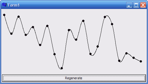
Using the Code
Here, I included CRSpline class and populates it with
pseudo-random control points, then uses BDS's TCanvas
interface to plot the spline on a regular dialog box's canvas.
I hope you did not find my little math session too boring. Enjoy the code.
References
- Computer Graphics: Principles and Practice; Foley, van Dam, Feiner, Hughes; Addison-Wesley, 1997
- Catmull, E. and R. Rom, "A Class of Local Interpolating Splines"; Computer-Aided Geometric Design; Academic Press, San Francisco, 1974
History
- 7th November, 2008: Initial post
License
This article, along with any associated source code and files, is licensed under The Code Project Open License (CPOL)
![]() 喜欢
喜欢
0
![]() 赠金笔
赠金笔