 加载中…
加载中…LaTeX和STATA
标签:
it |
分类: Latex |
Stata 与LaTeX 和 Word
的完美结合
Introductory examples for esttab
- Basic syntax and usage
- Standard errors, p-values, and summary statistics
- Beta coefficients
- Wide table: coefficients and t-statistics side-by-side
- Numerical formats
- Labels, titles, and notes
- Plain table
- Compressed table
- Significance stars: change symbols and thresholds
- Use with Excel
- Use with Word
- Use with LaTeX
- Non-standard table contents
-
Viewing the
internal
estout call
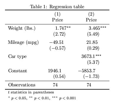
Basic syntax and usage
esttab
esttab [ namelist ] [ using filename ] [ , options estout_options ]
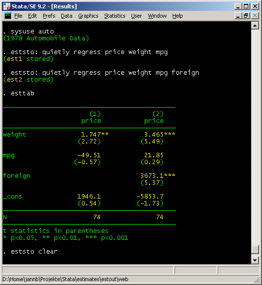
The procedure is to first store a number of models and then
apply
. sysuse auto
(1978 Automobile Data)

. eststo: quietly regress price weight mpg
(est1 stored)

. eststo: quietly regress price weight mpg foreign
(est2 stored)

. esttab

--------------------------------------------
                      (1)             (2)
                    price           price
--------------------------------------------
weight              1.747**         3.465***
                   (2.72)          (5.49)

mpg                -49.51           21.85
                  (-0.57)          (0.29)

foreign                            3673.1***
                                   (5.37)

_cons              1946.1         -5853.7
                   (0.54)         (-1.73)
--------------------------------------------
N                      74              74
--------------------------------------------
t statistics in parentheses
* p<0.05, ** p<0.01, *** p<0.001

. eststo clear


[do-file]
Note that the dashed lines appear as solid lines in Stata's results window:
http://repec.org/bocode/e/estout/esttab001.png
Standard errors, p-values, and summary statistics
The default in
. sysuse auto
(1978 Automobile Data)

. eststo: quietly regress price weight mpg
(est1 stored)

. eststo: quietly regress price weight mpg foreign
(est2 stored)

. esttab, se ar2

--------------------------------------------
                      (1)             (2)
                    price           price
--------------------------------------------
weight              1.747**         3.465***
                  (0.641)         (0.631)

mpg                -49.51           21.85
                  (86.16)         (74.22)

foreign                            3673.1***
                                  (684.0)

_cons              1946.1         -5853.7
                 (3597.0)        (3377.0)
--------------------------------------------
N                      74              74
adj. R-sq           0.273           0.478
--------------------------------------------
Standard errors in parentheses
* p<0.05, ** p<0.01, *** p<0.001


[do-file]
The t-statistics can also be replaced by p-values (p),
confidence intervals (ci), or any parameter statistics
contained in the estimates (see the
. esttab, p scalars(F df_m df_r)

--------------------------------------------
                      (1)             (2)
                    price           price
--------------------------------------------
weight              1.747**         3.465***
                  (0.008)         (0.000)

mpg                -49.51           21.85
                  (0.567)         (0.769)

foreign                            3673.1***
                                  (0.000)

_cons              1946.1         -5853.7
                  (0.590)         (0.087)
--------------------------------------------
N                      74              74
F                   14.74           23.29
df_m                    2               3
df_r                   71              70
--------------------------------------------
p-values in parentheses
* p<0.05, ** p<0.01, *** p<0.001

. eststo clear


[do-file]
Beta coefficients
To display beta coefficients and suppress the t-statistics type:
. sysuse auto
(1978 Automobile Data)

. eststo: quietly regress price weight mpg
(est1 stored)

. eststo: quietly regress price weight mpg foreign
(est2 stored)

. esttab, beta not

--------------------------------------------
                      (1)             (2)
                    price           price
--------------------------------------------
weight              0.460**         0.913***
mpg                -0.097           0.043
foreign                             0.573***
--------------------------------------------
N                      74              74
--------------------------------------------
Standardized beta coefficients
* p<0.05, ** p<0.01, *** p<0.001

. eststo clear


[do-file]
Wide table: coefficients and t-statistics side-by-side
The
. sysuse auto
(1978 Automobile Data)

. eststo: quietly regress price weight mpg
(est1 stored)

. eststo: quietly regress price weight mpg foreign
(est2 stored)

. esttab, wide

----------------------------------------------------------------------
                      (1)                          (2)
                    price                        price
----------------------------------------------------------------------
weight              1.747**        (2.72)        3.465***       (5.49)
mpg                -49.51         (-0.57)        21.85          (0.29)
foreign                                         3673.1***       (5.37)
_cons              1946.1          (0.54)      -5853.7         (-1.73)
----------------------------------------------------------------------
N                      74                           74
----------------------------------------------------------------------
t statistics in parentheses
* p<0.05, ** p<0.01, *** p<0.001

. eststo clear


[do-file]
Numerical formats
esttab
The format applied to a certain statistic can be changed by adding the appropriate display format specification in parentheses. For example, to increase precision for the point estimates and display p-values and the R-squared using four decimal places, type:
. sysuse auto
(1978 Automobile Data)

. eststo: quietly regress price weight mpg
(est1 stored)

. eststo: quietly regress price weight mpg foreign
(est2 stored)

. esttab, b(a6) p(4) r2(4) nostar wide

----------------------------------------------------------------
                      (1)                       (2)
                    price                     price
----------------------------------------------------------------
weight           1.746559     (0.0081)     3.464706     (0.0000)
mpg             -49.51222     (0.5673)     21.85360     (0.7693)
foreign                                    3673.060     (0.0000)
_cons            1946.069     (0.5902)    -5853.696     (0.0874)
----------------------------------------------------------------
N                      74                        74
R-sq               0.2934                    0.4996
----------------------------------------------------------------
p-values in parentheses

. eststo clear


[do-file]
Available formats are official Stata's display formats, such as
%9.0g or %8.2f (see helpformat).
Alternatively, as is illustrated in the example above, a fixed
format can be requested by specifying a single integer indicating
the desired number of decimal places. Furthermore, an adaptive
format a# may be specified, where # determines the minimum number
of "significant digits" to be printed (# should be in {1,2,...,9})
(see the
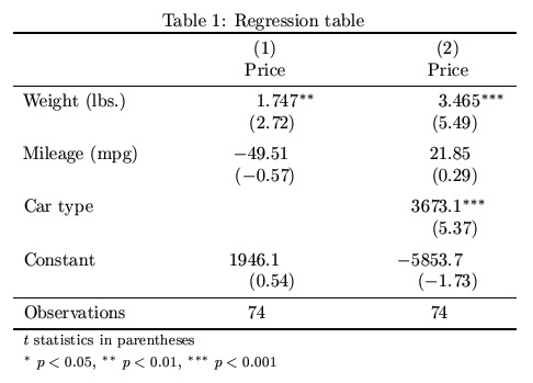
Labels, titles, and notes
To use variable labels and add some titles and notes, e.g., type:
. sysuse auto
(1978 Automobile Data)

. eststo: quietly regress price weight mpg
(est1 stored)

. eststo: quietly regress price weight mpg foreign
(est2 stored)

. esttab, label                               ///
>     title(This is a regression table)       ///
>     nonumbers mtitles("Model A" "Model B")  ///
>     addnote("Source: auto.dta")

This is a regression table
----------------------------------------------------
                          Model A         Model B
----------------------------------------------------
Weight (lbs.)               1.747**         3.465***
                           (2.72)          (5.49)

Mileage (mpg)              -49.51           21.85
                          (-0.57)          (0.29)

Car type                                   3673.1***
                                           (5.37)

Constant                   1946.1         -5853.7
                           (0.54)         (-1.73)
----------------------------------------------------
Observations                   74              74
----------------------------------------------------
t statistics in parentheses
Source: auto.dta
* p<0.05, ** p<0.01, *** p<0.001

. eststo clear


[do-file]
The label option supports factor variables and interactions in Stata 11 or newer:
. sysuse auto
(1978 Automobile Data)

. eststo: quietly regress price mpg i.foreign
(est1 stored)

. eststo: quietly regress price c.mpg##i.foreign
(est2 stored)

. esttab, varwidth(25)

---------------------------------------------------------
                                   (1)             (2)
                                 price           price
---------------------------------------------------------
mpg                             -294.2***       -329.3***
                               (-5.28)         (-4.39)

0.foreign                            0               0
                                   (.)             (.)

1.foreign                       1767.3*         -13.59
                                (2.52)         (-0.01)

0.foreign#c.mpg                                      0
                                                   (.)

1.foreign#c.mpg                                  78.89
                                                (0.70)

_cons                          11905.4***      12600.5***
                               (10.28)          (8.25)
---------------------------------------------------------
N                                   74              74
---------------------------------------------------------
t statistics in parentheses
* p<0.05, ** p<0.01, *** p<0.001

. esttab, varwidth(25) label

---------------------------------------------------------
                                   (1)             (2)
                                 Price           Price
---------------------------------------------------------
Mileage (mpg)                   -294.2***       -329.3***
                               (-5.28)         (-4.39)

Domestic                             0               0
                                   (.)             (.)

Foreign                         1767.3*         -13.59
                                (2.52)         (-0.01)

Domestic # Mileage (mpg)                             0
                                                   (.)

Foreign # Mileage (mpg)                          78.89
                                                (0.70)

Constant                       11905.4***      12600.5***
                               (10.28)          (8.25)
---------------------------------------------------------
Observations                        74              74
---------------------------------------------------------
t statistics in parentheses
* p<0.05, ** p<0.01, *** p<0.001

. esttab, varwidth(25) label nobaselevels interaction(" X ")

---------------------------------------------------------
                                   (1)             (2)
                                 Price           Price
---------------------------------------------------------
Mileage (mpg)                   -294.2***       -329.3***
                               (-5.28)         (-4.39)

Foreign                         1767.3*         -13.59
                                (2.52)         (-0.01)

Foreign X Mileage (mpg)                          78.89
                                                (0.70)

Constant                       11905.4***      12600.5***
                               (10.28)          (8.25)
---------------------------------------------------------
Observations                        74              74
---------------------------------------------------------
t statistics in parentheses
* p<0.05, ** p<0.01, *** p<0.001

. eststo clear


[do-file]
Plain table
The
. sysuse auto
(1978 Automobile Data)

. eststo: quietly regress price weight mpg
(est1 stored)

. eststo: quietly regress price weight mpg foreign
(est2 stored)

. esttab, plain

                     est1         est2
                      b/t          b/t
weight           1.746559     3.464706
                 2.723238     5.493003
mpg             -49.51222      21.8536
                -.5746808     .2944391
foreign                        3673.06
                              5.370142
_cons            1946.069    -5853.696
                  .541018    -1.733408
N                      74           74

. eststo clear


[do-file]
Compressed table
The
. sysuse auto
(1978 Automobile Data)

. eststo: quietly regress price weight
(est1 stored)

. eststo: quietly regress price weight mpg
(est2 stored)

. eststo: quietly regress price weight mpg foreign
(est3 stored)

. eststo: quietly regress price weight mpg foreign displacement
(est4 stored)

. esttab, compress

--------------------------------------------------------------
                 (1)          (2)          (3)          (4)
               price        price        price        price
--------------------------------------------------------------
weight         2.044***     1.747**      3.465***     2.458**
              (5.42)       (2.72)       (5.49)       (2.82)

mpg                        -49.51        21.85        19.08
                          (-0.57)       (0.29)       (0.26)

foreign                                 3673.1***    3930.2***
                                        (5.37)       (5.67)

displace~t                                            10.22
                                                     (1.65)

_cons         -6.707       1946.1      -5853.7      -4846.8
             (-0.01)       (0.54)      (-1.73)      (-1.43)
--------------------------------------------------------------
N                 74           74           74           74
--------------------------------------------------------------
t statistics in parentheses
* p<0.05, ** p<0.01, *** p<0.001

. eststo clear


[do-file]
Significance stars: change symbols and thresholds
The default symbols and thresholds are for the "significance stars" are: * for p<.05, ** for p<.01, and *** for p<.001. To use + for p<.10 and * for p<.05, for example, type:
. sysuse auto
(1978 Automobile Data)

. eststo: quietly regress price weight mpg
(est1 stored)

. eststo: quietly regress price weight mpg foreign
(est2 stored)

. esttab, star(+ 0.10 * 0.05)

----------------------------------------
                      (1)           (2)
                    price         price
----------------------------------------
weight              1.747*        3.465*
                   (2.72)        (5.49)

mpg                -49.51         21.85
                  (-0.57)        (0.29)

foreign                          3673.1*
                                 (5.37)

_cons              1946.1       -5853.7+
                   (0.54)       (-1.73)
----------------------------------------
N                      74            74
----------------------------------------
t statistics in parentheses
+ p<0.10, * p<0.05

. eststo clear


[do-file]
Use the
Use with Excel
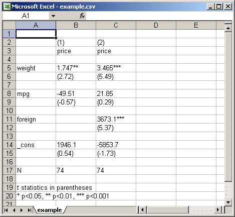
To produce a table for use with Excel, specify an output filename
and apply the
. sysuse auto
(1978 Automobile Data)

. eststo: quietly regress price weight mpg
(est1 stored)

. eststo: quietly regress price weight mpg foreign
(est2 stored)

. esttab using example.csv
(output written to example.csv)


[do-file]
A click on "example.csv" in Stata's results window will launch Excel and display the file:
http://repec.org/bocode/e/estout/esttab010.png
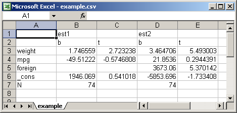
Depending on whether the
. esttab using example.csv, replace wide plain
(output written to example.csv)

. eststo clear


[do-file]
Result:
http://repec.org/bocode/e/estout/esttab010b.png
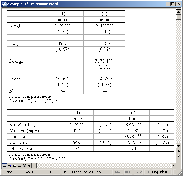
Use with Word
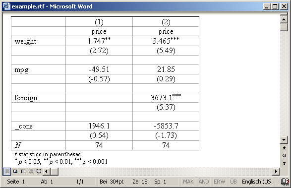
To produce a table for use with Word, specify an output filename
with an
. sysuse auto
(1978 Automobile Data)

. eststo: quietly regress price weight mpg
(est1 stored)

. eststo: quietly regress price weight mpg foreign
(est2 stored)

. esttab using example.rtf
(output written to example.rtf)


[do-file]
Result:
http://repec.org/bocode/e/estout/esttab011.png
Appending is possible.
Furthermore,
. esttab using example.rtf, append wide label modelwidth(8)
(output written to example.rtf)


[do-file]
Result:
http://repec.org/bocode/e/estout/esttab011b.png
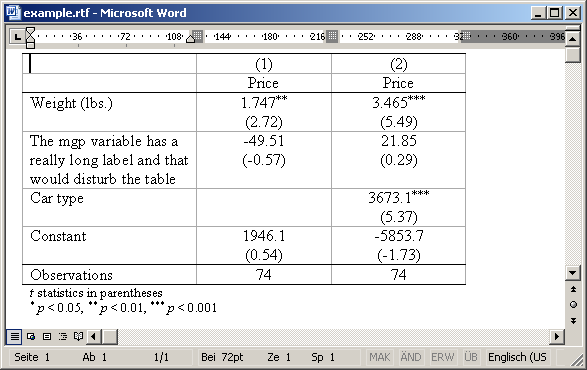
Another very useful feature is the
. lab var mpg "The mgp variable has a really long label and that would disturb
> the table"

. esttab using example.rtf, replace label nogap onecell
(output written to example.rtf)


[do-file]
Result:
http://repec.org/bocode/e/estout/esttab011c.png
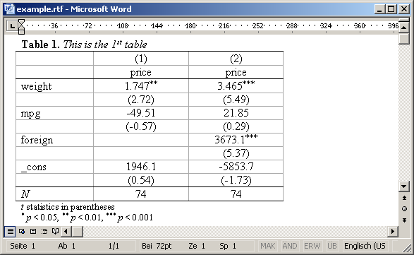
If you know a bit RTF you can also include RTF commands to achieve specific effects, although you have to be careful not to break the document (most importantly, do not introduce unmatched curly braces). Useful are, for example, "{\b ...}" for boldface and "{\i ...}" for italics. A very helpful reference is the "RTF Pocket Guide" by Sean M. Burke (O'Reilly). Example
. esttab using example.rtf, replace nogaps ///
>     title({\b Table 1.} {\i This is the 1{\super st} table})
(output written to example.rtf)


[do-file]
Result:
http://repec.org/bocode/e/estout/esttab011d.png
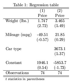
Use with LaTeX
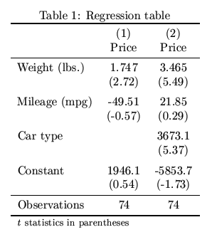
To create a table to be included in a LaTeX document, type:
. sysuse auto
(1978 Automobile Data)

. eststo: quietly regress price weight mpg
(est1 stored)

. eststo: quietly regress price weight mpg foreign
(est2 stored)

. esttab using example.tex, label nostar ///
>   title(Regression table\label{tab1})
(output written to example.tex)


[do-file]
TeXifying a document containing
\documentclass{article}
\begin{document}
\input{example.tex}
\end{document}
then produces the following result:
http://repec.org/bocode/e/estout/esttab012.png
Note
that
The table above looks alright, but a better result is achieved by
specifying the
. esttab using example.tex, label nostar replace booktabs ///
>   title(Regression table\label{tab1})
(output written to example.tex)


[do-file]
Result:
http://repec.org/bocode/e/estout/esttab012b.png
A further improvement is to load LaTeX's
. esttab using example.tex, label replace booktabs ///
>   alignment(D{.}{.}{-1})                         ///
>   title(Regression table\label{tab1})
(output written to example.tex)


[do-file]
Result:
http://repec.org/bocode/e/estout/esttab012c.png
Last but not least, it might be reasonable to space the table out to a certain width:
. esttab using example.tex, label replace booktabs ///
>   alignment(D{.}{.}{-1}) width(0.8\hsize)        ///
>   title(Regression table\label{tab1})
(output written to example.tex)

. eststo clear


[do-file]
Result:
http://repec.org/bocode/e/estout/esttab012d.png
Non-standard table contents
Sometimes it is necessary to include parameter statistics in a
table for which no predefined option exists
in
. sysuse auto
(1978 Automobile Data)

. quietly regress price weight mpg foreign

. estadd vif

    Variable |       VIF       1/VIF
-------------+----------------------
      weight |      3.86    0.258809
         mpg |      2.96    0.337297
     foreign |      1.59    0.627761
-------------+----------------------
    Mean VIF |      2.81

added matrix:
                e(vif) :  1 x 4

. esttab, aux(vif 2) wide nopar

-----------------------------------------
                      (1)
                    price
-----------------------------------------
weight              3.465***         3.86
mpg                 21.85            2.96
foreign            3673.1***         1.59
_cons             -5853.7
-----------------------------------------
N                      74
-----------------------------------------
vif in second column
* p<0.05, ** p<0.01, *** p<0.001


[do-file]
(Note: The second argument
in
However, if you want to include more than two kinds of parameter
statistics, you have to switch
to
. sysuse auto
(1978 Automobile Data)

. quietly regress price weight mpg foreign

. estadd vif

    Variable |       VIF       1/VIF
-------------+----------------------
      weight |      3.86    0.258809
         mpg |      2.96    0.337297
     foreign |      1.59    0.627761
-------------+----------------------
    Mean VIF |      2.81

added matrix:
                e(vif) :  1 x 4

. esttab, cells("b(fmt(a3) star) vif(fmt(2))" t(par fmt(2)))

-----------------------------------------
                      (1)
                    price
                      b/t             vif
-----------------------------------------
weight              3.465***         3.86
                   (5.49)
mpg                 21.85            2.96
                   (0.29)
foreign            3673.1***         1.59
                   (5.37)
_cons             -5853.7
                  (-1.73)
-----------------------------------------
N                      74
-----------------------------------------


[do-file]
Similarly, for a complicated summary statistics section in the
table footer you might have to
useestout's
Viewing the
internal estout call
Sometimes, an approach is to
use
. sysuse auto
(1978 Automobile Data)

. eststo: quietly regress price weight mpg
(est1 stored)

. eststo: quietly regress price weight mpg foreign
(est2 stored)

. esttab, noisily notype
estout ,
 cells(b(fmt(a3) star) t(fmt(2) par("{ralign @modelwidth:{txt:(}" "{txt:)}}")))
 stats(N, fmt(.0g) labels(`"N"'))
 starlevels(* 0.05 ** 0.01 *** 0.001)
 varwidth(12)
 modelwidth(12)
 abbrev
 delimiter(" ")
 smcltags
 prehead(`"{hline @width}"')
 posthead("{hline @width}")
 prefoot("{hline @width}")
 postfoot(`"{hline @width}"' `"t statistics in parentheses"' `"@starlegend"')
 varlabels(, end("" "") nolast)
 mlabels(, depvar)
 numbers
 collabels(none)
 eqlabels(, begin("{hline @width}" "") nofirst)
 interaction(" # ")
 notype
 level(95)
 style(esttab)

. return list

scalars:
            r(nmodels) =  2
              r(ccols) =  3

macros:
              r(names) : "est1 est2"
         r(m2_depname) : "price"
         r(m1_depname) : "price"
            r(cmdline) : "estout , cells(b(fmt(a3) star) t(fmt(2) par("{ral.."

matrices:
              r(coefs) :  4 x 6
              r(stats) :  1 x 2

. eststo clear


[do-file]
(notype
![]() 喜欢
喜欢
0
![]() 赠金笔
赠金笔