 加载中…
加载中…Logistic regression (逻辑回归) 概述
标签:
logisticregressionit |
分类: MachineLearning |
Logistic regression (逻辑回归) 概述
Logistic
http://hiphotos.baidu.com/hehehehello/pic/item/b81c5cb56260e19137d3ca76.jpgregression
http://hiphotos.baidu.com/hehehehello/pic/item/70c8710982bc58f02fddd476.jpgregression
http://bits.wikimedia.org/skins-1.17/common/images/magnify-clip.pngregression
三、Logistic
1)
2)
3)
转自: http://hi.baidu.com/hehehehello/item/40025c33d7d9b7b9633aff87
第一个matlab程序 Logistic Regression
如果预测值只能是0或者1,线性回归不是一个好的办法,线性回归不能把输出值限制在区间(0,1)。
那么可以做一个logistic变换,使得变换之后的输出值区间限制在(0,1)。
http://f.hiphotos.baidu.com/space/pic/item/dc54564e9258d1094eea342dd158ccbf6c814d20.jpgregression
是一个关于(0,0.5)对称的奇函数。
http://h.hiphotos.baidu.com/space/pic/item/9358d109b3de9c822e3b64106c81800a18d843d7.jpgregression
假设
http://e.hiphotos.baidu.com/space/pic/item/b21bb051f81986185210721b4aed2e738ad4e6de.jpgregression
则
http://b.hiphotos.baidu.com/space/pic/item/6a63f6246b600c33262943571a4c510fd8f9a1d9.jpgregression
求其似然函数:
http://c.hiphotos.baidu.com/space/pic/item/a1ec08fa513d2697d36195c255fbb2fb4216d8fb.jpgregression
log似然函数:
http://e.hiphotos.baidu.com/space/pic/item/d833c895d143ad4b95b4db5f82025aafa50f0692.jpgregression
最大似然要使其log似然函数值最大,用梯度下降法求取最大值时的参数。
http://d.hiphotos.baidu.com/space/pic/item/48540923dd54564e69b679a6b3de9c82d0584f5a.jpgregression
最终迭代更新参数的公式为:
http://g.hiphotos.baidu.com/space/pic/item/b7fd5266d01609249dfa3f84d40735fae7cd3455.jpgregression
在matlab上简单实现了下,主要是为了熟悉matlab的语法及函数。
function
xSize
xRowSize
xColSize
�d
%this
onesColum
X=[onesColum,X];
ySize
yRowSize
yColSize
%check
if
end
if
end
%initialize
thetaSize
theta
esp
loss
iter
maxIter
while
end
display(sprintf('iter
end
>>
>>
>>
iter
B
>>
C
可以看出来B和C的值接近。
转自: http://hi.baidu.com/flower_mlh/item/a148bfd8a9b1ab13d78ed002
Stanford机器学习---第三讲. 逻辑回归和过拟合问题的解决 logistic Regression & Regularization
本栏目(Machine learning)包括单参数的线性回归、多参数的线性回归、Octave Tutorial、Logistic Regression、Regularization、神经网络、机器学习系统设计、SVM(Support Vector Machines 支持向量机)、聚类、降维、异常检测、大规模机器学习等章节。所有内容均来自Standford公开课machine learning中Andrew老师的讲解。(https://class.coursera.org/ml/class/index)
第三讲-------Logistic Regression & Regularization
本讲内容:
Logistic Regression
=========================
(一)、Classification
(二)、Hypothesis Representation
(三)、Decision Boundary
(四)、Cost Function
(五)、Simplified Cost Function and Gradient Descent
(六)、Parameter Optimization in Matlab
(七)、Multiclass classification : One-vs-all
The problem of
overfitting and how to solve
it
=========================
(八)、The problem of overfitting
(九)、Cost Function
(十)、Regularized Linear Regression
(十一)、Regularized Logistic Regression
本章主要讲述逻辑回归和Regularization解决过拟合的问题,非常非常重要,是机器学习中非常常用的回归工具,下面分别进行两部分的讲解。
第一部分:Logistic Regression
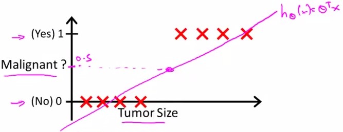
假设随Tumor Size变化,预测病人的肿瘤是恶性(malignant)还是良性(benign)的情况。
给出8个数据如下:
假设进行linear regression得到的hypothesis线性方程如上图中粉线所示,则可以确定一个threshold:0.5进行predict
y=1, if h(x)>=0.5
y=0, if
即malignant=0.5的点投影下来,其右边的点预测y=1;左边预测y=0;则能够很好地进行分类。
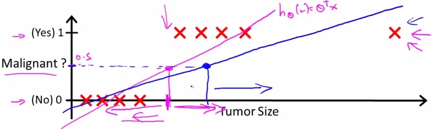
那么,如果数据集是这样的呢?
http://my.csdn.net/uploads/201207/04/1341403402_9129.jpgregression
这种情况下,假设linear regression预测为蓝线,那么由0.5的boundary得到的线性方程中,不能很好地进行分类。因为不满足
y=1, h(x)>0.5
y=0, h(x)<=0.5
这时,我们引入logistic regression model:
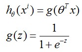
http://my.csdn.net/uploads/201207/04/1341403634_5914.jpgregression
所谓Sigmoid function或Logistic function就是这样一个函数g(z)见上图所示
当z>=0时,g(z)>=0.5;当z<0时,g(z)<0.5
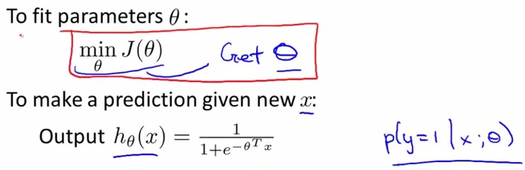
由下图中公式知,给定了数据x和参数θ,y=0和y=1的概率和=1
http://my.csdn.net/uploads/201207/04/1341404302_5369.jpgregression
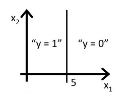
所谓Decision Boundary就是能够将所有数据点进行很好地分类的h(x)边界。
如下图所示,假设形如h(x)=g(θ0+θ1x1+θ2x2)的hypothesis参数θ=[-3,1,1]T, 则有
predict Y=1, if -3+x1+x2>=0
predict Y=0, if -3+x1+x2<0
刚好能够将图中所示数据集进行很好地分类
http://my.csdn.net/uploads/201207/05/1341470683_7505.jpgregression
Another Example:
http://my.csdn.net/uploads/201207/05/1341471264_6699.jpgregression
answer:
http://my.csdn.net/uploads/201207/05/1341471309_5596.jpgregression
除了线性boundary还有非线性decision
boundaries,比如http://my.csdn.net/uploads/201207/05/1341472718_8627.jpgregression
下图中,进行分类的decision boundary就是一个半径为1的圆,如图所示:
http://my.csdn.net/uploads/201207/05/1341471338_7289.jpgregression
该部分讲述简化的logistic regression系统中how to implement gradient descents for logistic regression.
假设我们的数据点中y只会取0和1,
对于一个logistic regression model系统,有http://my.csdn.net/uploads/201207/07/1341657968_4370.jpgregression
http://my.csdn.net/uploads/201207/07/1341650794_3936.jpgregression
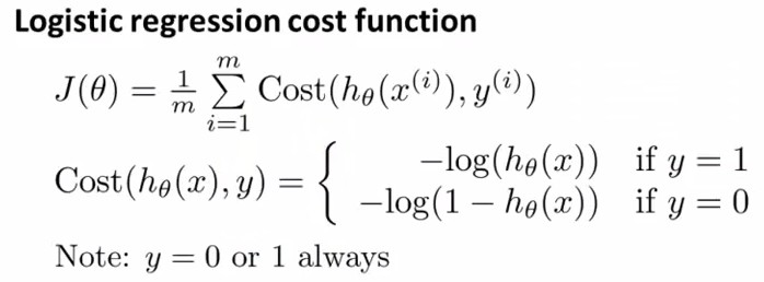
由于y只会取0,1,那么就可以写成
http://my.csdn.net/uploads/201207/07/1341658176_1292.jpgregression
不信的话可以把y=0,y=1分别代入,可以发现这个J(θ)和上面的Cost(hθ(x),y)是一样的(*^__^*) ,那么剩下的工作就是求能最小化 J(θ)的θ了~
http://my.csdn.net/uploads/201207/07/1341658365_6677.jpgregression
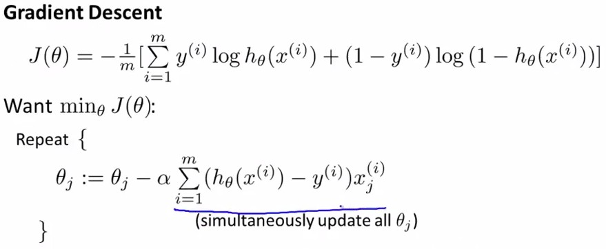
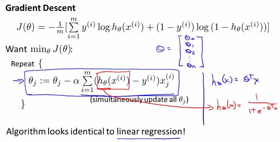
在第一章中我们已经讲了如何应用Gradient Descent, 也就是下图Repeat中的部分,将θ中所有维同时进行更新,而J(θ)的导数可以由下面的式子求得,结果如下图手写所示:
http://my.csdn.net/uploads/201207/07/1341658423_4153.jpgregression
现在将其带入Repeat中:
http://my.csdn.net/uploads/201207/07/1341658851_7555.jpgregression
这是我们惊奇的发现,它和第一章中我们得到的公式http://my.csdn.net/uploads/201207/07/1341650756_4768.jpgregression
也就是说,下图中所示,不管h(x)的表达式是线性的还是logistic regression model, 都能得到如下的参数更新过程。
http://my.csdn.net/uploads/201207/07/1341659008_4711.jpgregression
那么如何用vectorization来做呢?换言之,我们不要用for循环一个个更新θj,而用一个矩阵乘法同时更新整个θ。也就是解决下面这个问题:
http://my.csdn.net/uploads/201207/07/1341659160_9211.jpgregression
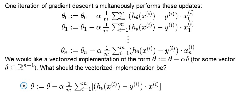
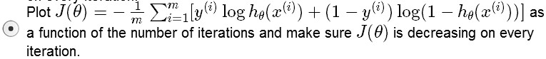
上面的公式给出了参数矩阵θ的更新,那么下面再问个问题,第二讲中说了如何判断学习率α大小是否合适,那么在logistic regression系统中怎么评判呢?
Q:Suppose you are running gradient descent to
fit a logistic regression model with
parameter
A:http://my.csdn.net/uploads/201207/07/1341659914_3644.jpgregression
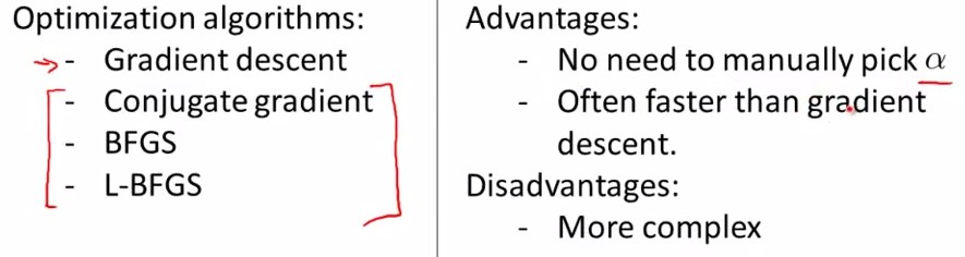
这部分内容将对logistic regression 做一些优化措施,使得能够更快地进行参数梯度下降。本段实现了matlab下用梯度方法计算最优参数的过程。
首先声明,除了gradient descent 方法之外,我们还有很多方法可以使用,如下图所示,左边是另外三种方法,右边是这三种方法共同的优缺点,无需选择学习率α,更快,但是更复杂。
http://my.csdn.net/uploads/201207/07/1341662451_8533.jpgregression
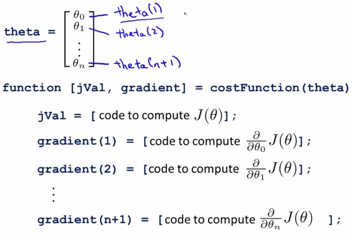
也就是matlab中已经帮我们实现好了一些优化参数θ的方法,那么这里我们需要完成的事情只是写好cost
function,并告诉系统,要用哪个方法进行最优化参数。比如我们用‘GradObj’,
http://my.csdn.net/uploads/201207/07/1341662943_3392.jpgregression
如上图所示,给定了参数θ,我们需要给出cost Function.
其中,
jVal 是 cost function
的表示,比如设有两个点(1,0,5)和(0,1,5)进行回归,那么就设方程为hθ(x)=θ1x1+θ2x2;
则有costfunction J(θ):
jVal=(theta(1)-5)^2+(theta(2)-5)^2;
在每次迭代中,按照gradient
descent的方法更新参数θ:θ(i)-=gradient(i),其中gradient(i)是J(θ)对θi求导的函数式,在此例中就有gradient(1)=2*(theta(1)-5),
函数costFunction, 定义jVal=J(θ)和对两个θ的gradient:
-
function
[ jVal,gradient ] = costFunction( theta ) -
%COSTFUNCTION
Summary thisof function goes here -
%
Detailed explanation goes here -
-
jVal=
(theta(1)-5)^2+(theta(2)-5)^2; -
-
gradient
= zeros(2,1); -
%code
to compute derivative to theta -
gradient(1)
= 2 * (theta(1)-5); -
gradient(2)
= 2 * (theta(2)-5); -
- end
编写函数Gradient_descent,进行参数优化
-
function
[optTheta,functionVal,exitFlag]=Gradient_descent( ) -
%GRADIENT_DESCENT
Summary thisof function goes here -
%
Detailed explanation goes here -
-
options 'GradObj','on','MaxIter',100);= optimset( -
initialTheta = zeros(2,1) -
[optTheta,functionVal,exitFlag] = fminunc(@costFunction,initialTheta,options); -
-
end
matlab主窗口中调用,得到优化厚的参数(θ1,θ2)=(5,5),即hθ(x)=θ1x1+θ2x2=5*x1+5*x2
-
[optTheta,functionVal,exitFlag] = Gradient_descent() -
-
initialTheta
= -
-
0 -
0 -
-
-
Local
minimum found. -
-
Optimization
completed because the size of the gradient is less than - the
default value of the function tolerance. -
-
-
-
-
optTheta
= -
-
5 -
5 -
-
-
functionVal
= -
-
0 -
-
-
exitFlag
= -
-
1
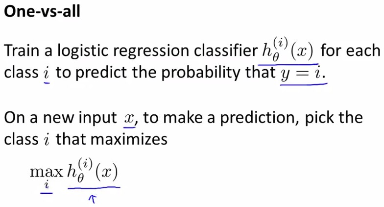
所谓one-vs-all method就是将binary分类的方法应用到多类分类中。
比如我想分成K类,那么就将其中一类作为positive,另(k-1)合起来作为negative,这样进行K个h(θ)的参数优化,每次得到的一个hθ(x)是指给定θ和x,它属于positive的类的概率。http://my.csdn.net/uploads/201207/07/1341665118_5132.jpgregression
按照上面这种方法,给定一个输入向量x,获得最大hθ(x)的类就是x所分到的类。
http://my.csdn.net/uploads/201207/07/1341665135_8657.jpgregression
第二部分:The problem of overfitting and how to solve
it
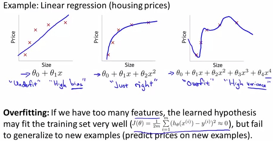
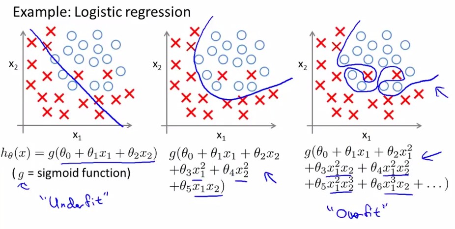
The Problem of overfitting:
overfitting就是过拟合,如下图中最右边的那幅图。对于以上讲述的两类(logistic regression和linear regression)都有overfitting的问题,下面分别用两幅图进行解释:
:
http://my.csdn.net/uploads/201207/09/1341813990_1647.jpgregression
:
http://my.csdn.net/uploads/201207/09/1341814477_1796.jpgregression
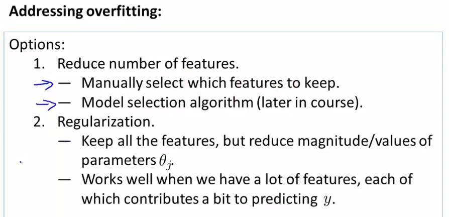
怎样解决过拟合问题呢?两个方法:
1. 减少feature个数(人工定义留多少个feature、算法选取这些feature)
2. 规格化(留下所有的feature,但对于部分feature定义其parameter非常小)
下面我们将对regularization进行详细的讲解。
http://my.csdn.net/uploads/201207/09/1341814873_5449.jpgregression
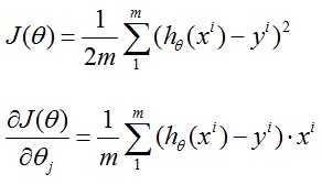
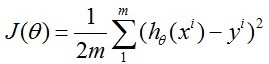
对于linear regression model, 我们的问题是最小化
写作矩阵表示即
i.e. the loss function can be written as
there we can get:
After regularization, however,we have:
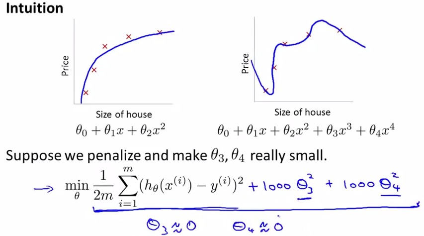
对于Regularization,方法如下,定义cost
function中θ3,θ4的parameter非常大,那么最小化cost
function后就有非常小的θ3,θ4了。
http://my.csdn.net/uploads/201207/09/1341819595_8466.jpgregression
写作公式如下,在cost function中加入θ1~θn的惩罚项:
http://my.csdn.net/uploads/201207/09/1341819852_5271.jpgregression
这里要注意λ的设置,见下面这个题目:
Q:http://my.csdn.net/uploads/201207/09/1341820005_6241.jpgregression
下面呢,我们分linear regression 和 logistic regression分别进行regularization步骤.
:
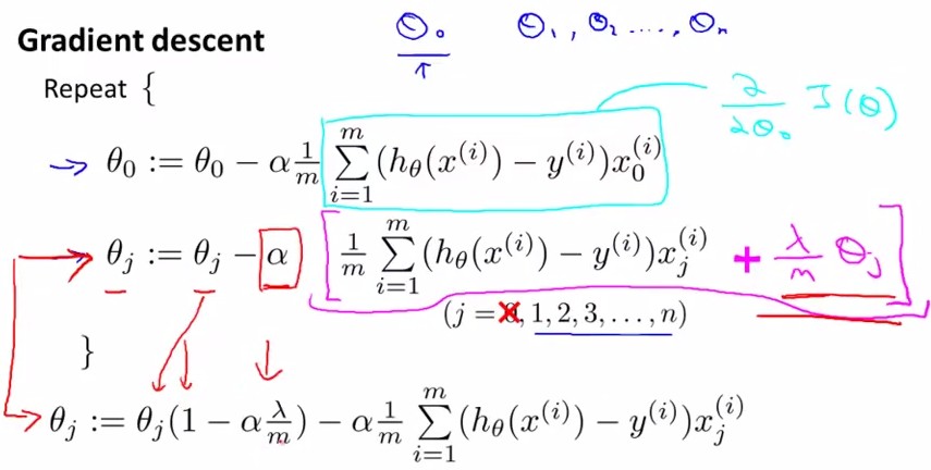
首先看一下,按照上面的cost function的公式,如何应用gradient descent进行参数更新。
对于θ0,没有惩罚项,更新公式跟原来一样
对于其他θj,J(θ)对其求导后还要加上一项(λ/m)*θj,见下图:
http://my.csdn.net/uploads/201207/09/1341820624_4372.jpgregression
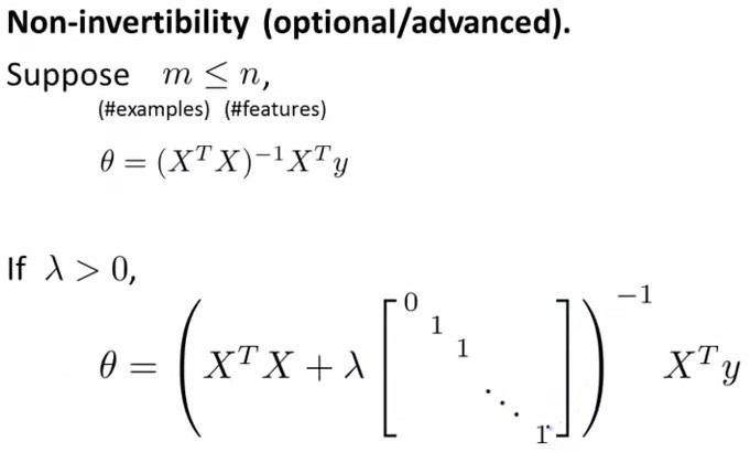
如果不使用梯度下降法(gradient descent+regularization),而是用矩阵计算(normal equation)来求θ,也就求使J(θ)min的θ,令J(θ)对θj求导的所有导数等于0,有公式如下:
http://my.csdn.net/uploads/201207/09/1341820647_5770.jpgregression
而且已经证明,上面公式中括号内的东西是可逆的。
:
前面已经讲过Logisitic Regression的cost function和overfitting的情况,如下图中所示:
http://my.csdn.net/uploads/201207/09/1341838465_5288.jpgregression
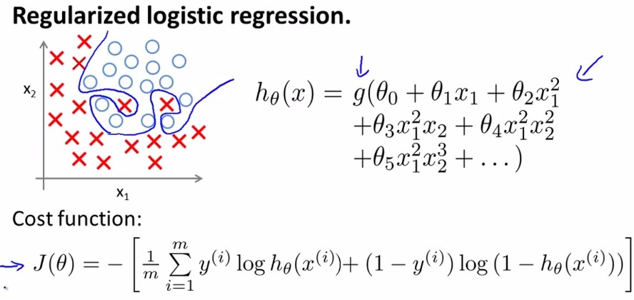
和linear regression一样,我们给J(θ)加入关于θ的惩罚项来抑制过拟合:(注意,不惩罚theta0,只惩罚其他项)
http://my.csdn.net/uploads/201207/09/1341838661_4509.jpgregression
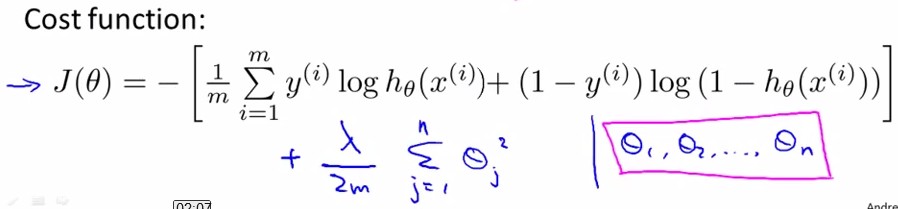
用Gradient Descent的方法,令J(θ)对θj求导都等于0,得到
http://my.csdn.net/uploads/201207/09/1341838835_1795.jpgregression
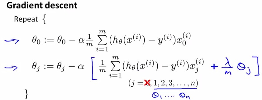
这里我们发现,其实和线性回归的θ更新方法是一样的。
When using
regularized logistic regression, which of these is the best way to
monitor whether gradient descent is working
correctly?
http://my.csdn.net/uploads/201207/09/1341837629_6163.jpgregression
和上面matlab中调用那个例子相似,我们可以定义logistic regression的cost function如下所示:
http://img.my.csdn.net/uploads/201207/09/1341839687_9495.jpgregression
图中,jval表示cost function 表达式,其中最后一项是参数θ的惩罚项;下面是对各θj求导的梯度,其中θ0没有在惩罚项中,因此gradient不变,θ1~θn分别多了一项(λ/m)*θj;
至此,regularization可以解决linear和logistic的overfitting regression问题了~
转自: http://blog.csdn.net/abcjennifer/article/details/7716281
Matlab实现线性回归和逻辑回归: Linear Regression & Logistic Regression
本文为Maching Learning
栏目补充内容,为上几章中所提到单参数线性回归、多参数线性回归和
本讲内容:
Matlab 实现各种回归函数
=========================
基本模型
Y=θ0+θ1X1型---线性回归(直线拟合)
解决过拟合问题---Regularization
Y=1/(1+e^X)型---逻辑回归(sigmod 函数拟合)
在解决拟合问题的解决之前,我们首先回忆一下线性回归和逻辑回归的基本模型。
设待拟合参数 θn*1 和输入参数[ xm*n, ym*1
]
对于各类拟合我们都要根据梯度下降的算法,给出两部分:
①
function [ jVal,gradient ] = costFunction ( theta )
②
function [optTheta,functionVal,exitFlag]=Gradient_descent( )
线性回归:拟合方程为hθ(x)=θ0x0+θ1x1+…+θnxn,当然也可以有xn的幂次方作为线性回归项(如http://my.csdn.net/uploads/201207/05/1341472718_8627.jpgregression
其cost function
为:http://my.csdn.net/uploads/201207/10/1341901237_1654.jpgregression
逻辑回归:拟合方程为hθ(x)=1/(1+e^(θTx)),其cost function 为:
http://my.csdn.net/uploads/201207/07/1341658176_1292.jpgregression
cost function对各θj的求导请自行求取,看第三章最后一图,或者参见后文代码。
后面,我们分别对几个模型方程进行拟合,给出代码,并用matlab中的fit函数进行验证。
在Matlab 线性拟合 & 非线性拟合中我们已经讲过如何用matlab自带函数fit进行直线和曲线的拟合,非常实用。而这里我们是进行ML课程的学习,因此研究如何利用前面讲到的梯度下降法(gradient descent)进行拟合。
-
function
[ jVal,gradient ] = costFunction2( theta ) -
%COSTFUNCTION2
Summary thisof function goes here -
%
linear regression -> y=theta0 + theta1*x -
%
parameter: x:m*n theta:n*1 y:m*1 (m=4,n=1) -
%
-
-
�ta
-
x=[1;2;3;4];
-
y=[1.1;2.2;2.7;3.8];
-
m=size(x,1);
-
-
hypothesis
= h_func(x,theta); -
delta
= hypothesis - y; -
jVal=sum(delta.^2);
-
-
gradient(1)=sum(delta)/m;
-
gradient(2)=sum(delta.*x)/m;
-
- end
其中,h_func是hypothesis的结果:
-
%H_FUNC
Summary thisof function goes here -
%
Detailed explanation goes here -
-
-
%cost
function 2 -
res=
theta(1)+theta(2)*inputx; -
function
[res] = h_func(inputx,theta) - end
-
function
[optTheta,functionVal,exitFlag]=Gradient_descent( ) -
%GRADIENT_DESCENT
Summary thisof function goes here -
%
Detailed explanation goes here -
-
options = optimset( -
initialTheta = zeros(2,1); -
[optTheta,functionVal,exitFlag] = fminunc(@costFunction2,initialTheta,options); -
-
end
function [optTheta,functionVal,exitFlag]=Gradient_descent( )
%GRADIENT_DESCENT Summary of this function goes here
%   Detailed explanation goes here

  options = optimset('GradObj','on','MaxIter',100);
  initialTheta = zeros(2,1);
  [optTheta,functionVal,exitFlag] = fminunc(@costFunction2,initialTheta,options);

end
result:
-
>>
[optTheta,functionVal,exitFlag] = Gradient_descent() -
-
Local
minimum found. -
-
Optimization
completed because the size of the gradient is less than - the
default value of the function tolerance. -
-
-
-
-
optTheta
= -
-
0.3000 -
0.8600 -
-
-
functionVal
= -
-
0.0720 -
-
-
exitFlag
= -
-
1
>> [optTheta,functionVal,exitFlag] = Gradient_descent()

Local minimum found.

Optimization completed because the size of the gradient is less than
the default value of the function tolerance.


optTheta =

    0.3000
    0.8600


functionVal =

    0.0720


exitFlag =

     1
-
function
[ parameter ] = checkcostfunc( ) -
%CHECKC2
Summary thisof function goes here -
%
check the cost function works well -
%
check with the matlab fit function as standard -
-
%check
cost function 2 -
x=[1;2;3;4];
-
y=[1.1;2.2;2.7;3.8];
-
- EXPR=
{ 'x','1'}; -
p=fittype(EXPR);
-
parameter=fit(x,y,p);
-
- end
function [ parameter ] = checkcostfunc(  )
%CHECKC2 Summary of this function goes here
%   check if the cost function works well
%   check with the matlab fit function as standard

%check cost function 2
x=[1;2;3;4];
y=[1.1;2.2;2.7;3.8];

EXPR= {'x','1'};
p=fittype(EXPR);
parameter=fit(x,y,p);

end
运行结果:
-
>>
checkcostfunc() -
-
ans
= -
-
Linear model: -
ans(x) = a*x + b -
Coefficients (with 95% confidence bounds): -
a = 0.86 (0.4949, 1.225) -
b = 0.3 (-0.6998, 1.3)
>> checkcostfunc()

ans =

     Linear model:
     ans(x) = a*x + b
     Coefficients (with 95% confidence bounds):
       a =        0.86  (0.4949, 1.225)
       b =         0.3  (-0.6998, 1.3)
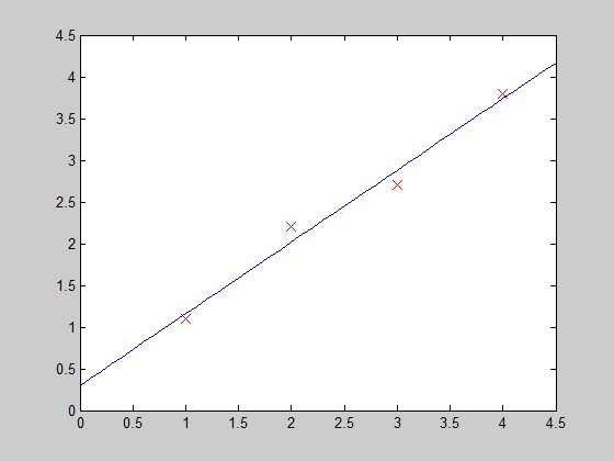
和我们的结果一样。下面画图:
-
function
PlotFunc( xstart,xend ) -
%PLOTFUNC
Summary thisof function goes here -
%
draw original data and the fitted -
-
-
-
%===================cost
function 2====linear regression -
%original
data -
x1=[1;2;3;4];
-
y1=[1.1;2.2;2.7;3.8];
- %plot(x1,y1,'ro-','MarkerSize',10);
- plot(x1,y1,'rx','MarkerSize',10);
-
hold
on; -
-
%fitted
line - 拟合曲线 -
x_co=xstart:0.1:xend;
-
y_co=0.3+0.86*x_co;
- %plot(x_co,y_co,'g');
-
plot(x_co,y_co);
-
-
hold
off; - end
function PlotFunc( xstart,xend )
%PLOTFUNC Summary of this function goes here
%   draw original data and the fitted


%===================cost function 2====linear regression
%original data
x1=[1;2;3;4];
y1=[1.1;2.2;2.7;3.8];
%plot(x1,y1,'ro-','MarkerSize',10);
plot(x1,y1,'rx','MarkerSize',10);
hold on;

%fitted line - 拟合曲线
x_co=xstart:0.1:xend;
y_co=0.3+0.86*x_co;
%plot(x_co,y_co,'g');
plot(x_co,y_co);

hold off;
end
在每次迭代中,按照gradient
descent的方法更新参数θ:θ(i)-=gradient(i),其中gradient(i)是J(θ)对θi求导的函数式,在此例中就有gradient(1)=2*(theta(1)-5),
函数costFunction, 定义jVal=J(θ)和对两个θ的gradient:
-
function
[ jVal,gradient ] = costFunction( theta ) -
%COSTFUNCTION
Summary thisof function goes here -
%
Detailed explanation goes here -
-
jVal=
(theta(1)-5)^2+(theta(2)-5)^2; -
-
gradient
= zeros(2,1); -
%code
to compute derivative to theta -
gradient(1)
= 2 * (theta(1)-5); -
gradient(2)
= 2 * (theta(2)-5); -
- end
function [ jVal,gradient ] = costFunction( theta )
%COSTFUNCTION Summary of this function goes here
%   Detailed explanation goes here

jVal= (theta(1)-5)^2+(theta(2)-5)^2;

gradient = zeros(2,1);
%code to compute derivative to theta
gradient(1) = 2 * (theta(1)-5);
gradient(2) = 2 * (theta(2)-5);

end
Gradient_descent,进行参数优化
-
function
[optTheta,functionVal,exitFlag]=Gradient_descent( ) -
%GRADIENT_DESCENT
Summary thisof function goes here -
%
Detailed explanation goes here -
-
options 'GradObj','on','MaxIter',100);= optimset( -
initialTheta = zeros(2,1) -
[optTheta,functionVal,exitFlag] = fminunc(@costFunction,initialTheta,options); -
-
end
function [optTheta,functionVal,exitFlag]=Gradient_descent( )
%GRADIENT_DESCENT Summary of this function goes here
%   Detailed explanation goes here

 options = optimset('GradObj','on','MaxIter',100);
 initialTheta = zeros(2,1)
 [optTheta,functionVal,exitFlag] = fminunc(@costFunction,initialTheta,options);

end
matlab主窗口中调用,得到优化厚的参数(θ1,θ2)=(5,5)
-
[optTheta,functionVal,exitFlag] = Gradient_descent() -
-
initialTheta
= -
-
0 -
0 -
-
-
Local
minimum found. -
-
Optimization
completed because the size of the gradient is less than - the
default value of the function tolerance. -
-
-
-
-
optTheta
= -
-
5 -
5 -
-
-
functionVal
= -
-
0 -
-
-
exitFlag
= -
-
1
 [optTheta,functionVal,exitFlag] = Gradient_descent()

initialTheta =

     0
     0


Local minimum found.

Optimization completed because the size of the gradient is less than
the default value of the function tolerance.


optTheta =

     5
     5


functionVal =

     0


exitFlag =

     1
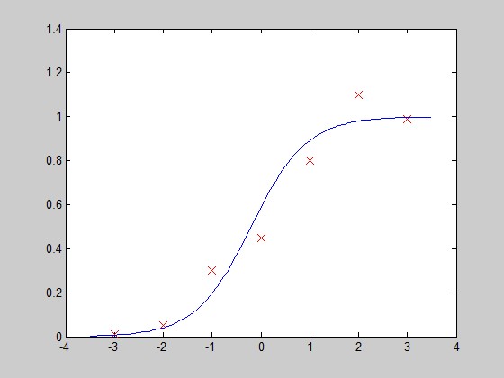
第四部分:Y=1/(1+e^X)型---逻辑回归(sigmod 函数拟合)
hypothesis function:-
function
[res] = h_func(inputx,theta) -
-
%cost
function 3 -
tmp=theta(1)+theta(2)*inputx;%m*1
-
res=1./(1+exp(-tmp));%m*1
-
-
end
function [res] = h_func(inputx,theta)

%cost function 3
tmp=theta(1)+theta(2)*inputx;%m*1
res=1./(1+exp(-tmp));%m*1

end
cost function:
-
function
[ jVal,gradient ] = costFunction3( theta ) -
%COSTFUNCTION3
Summary thisof function goes here -
%
Logistic Regression -
-
x=[-3;
-2; -1; 0; 1; 2; 3]; -
y=[0.01;
0.05; 0.3; 0.45; 0.8; 1.1; 0.99]; -
m=size(x,1);
-
-
%hypothesis
data -
hypothesis
= h_func(x,theta); -
-
%jVal-cost
function & gradient updating -
jVal=-sum(log(hypothesis+0.01).*y
+ (1-y).*log(1-hypothesis+0.01))/m; -
gradient(1)=sum(hypothesis-y)/m;
%reflect to theta1 -
gradient(2)=sum((hypothesis-y).*x)/m;
%reflect to theta 2 -
-
end
function [ jVal,gradient ] = costFunction3( theta )
%COSTFUNCTION3 Summary of this function goes here
%   Logistic Regression

x=[-3;      -2;     -1;     0;      1;      2;     3];
y=[0.01;    0.05;   0.3;    0.45;   0.8;    1.1;    0.99];
m=size(x,1);

%hypothesis  data
hypothesis = h_func(x,theta);

%jVal-cost function  &  gradient updating
jVal=-sum(log(hypothesis+0.01).*y + (1-y).*log(1-hypothesis+0.01))/m;
gradient(1)=sum(hypothesis-y)/m;   %reflect to theta1
gradient(2)=sum((hypothesis-y).*x)/m;    %reflect to theta 2

end
Gradient_descent:
-
function
[optTheta,functionVal,exitFlag]=Gradient_descent( ) -
-
options 'GradObj','on','MaxIter',100);= optimset( -
initialTheta = [0;0]; -
[optTheta,functionVal,exitFlag] = fminunc(@costFunction3,initialTheta,options); -
-
end
function [optTheta,functionVal,exitFlag]=Gradient_descent( )

 options = optimset('GradObj','on','MaxIter',100);
 initialTheta = [0;0];
 [optTheta,functionVal,exitFlag] = fminunc(@costFunction3,initialTheta,options);

end
运行结果:
-
[optTheta,functionVal,exitFlag] = Gradient_descent() -
-
Local
minimum found. -
-
Optimization
completed because the size of the gradient is less than - the
default value of the function tolerance. -
-
-
-
-
optTheta
= -
-
0.3526 -
1.7573 -
-
-
functionVal
= -
-
0.2498 -
-
-
exitFlag
= -
-
1
 [optTheta,functionVal,exitFlag] = Gradient_descent()

Local minimum found.

Optimization completed because the size of the gradient is less than
the default value of the function tolerance.


optTheta =

    0.3526
    1.7573


functionVal =

    0.2498


exitFlag =

     1
画图验证:
-
function
PlotFunc( xstart,xend ) -
%PLOTFUNC
Summary thisof function goes here -
%
draw original data and the fitted -
-
%===================cost
function 3=====logistic regression -
-
%original
data -
x=[-3;
-2; -1; 0; 1; 2; 3]; -
y=[0.01;
0.05; 0.3; 0.45; 0.8; 1.1; 0.99]; - plot(x,y,'rx','MarkerSize',10);
-
hold
on -
-
%fitted
line -
x_co=xstart:0.1:xend;
-
theta
= [0.3526,1.7573]; -
y_co=h_func(x_co,theta);
-
plot(x_co,y_co);
-
hold
off -
- end
function PlotFunc( xstart,xend )
%PLOTFUNC Summary of this function goes here
%   draw original data and the fitted

%===================cost function 3=====logistic regression

%original data
x=[-3;      -2;     -1;     0;      1;      2;     3];
y=[0.01;    0.05;   0.3;    0.45;   0.8;    1.1;    0.99];
plot(x,y,'rx','MarkerSize',10);
hold on

%fitted line
x_co=xstart:0.1:xend;
theta = [0.3526,1.7573];
y_co=h_func(x_co,theta);
plot(x_co,y_co);
hold off

end
![]() 喜欢
喜欢
0
![]() 赠金笔
赠金笔